A Simple 2D Model of Saturated Groundwater Flow in Permafrost Peatland Environments
2026-04-16
- hydrology
- modelling
- wildfire
- drought
Peat Plateau Groundwater Flow Simulator
A simple model of saturated subsurface flow through the supra-permafrost layer of northern peatlands, based on Darcy's Law and the depth-dependent hydraulic conductivity profile established by Quinton et al. (2008).
Legend
An Informal Introduction to Measuring Groundwater Flow Using Darcy's Law
It's important to clarify right off the bat that this model simulates groundwater flow in saturated conditions, but what does that actually mean? To start, let's establish some terminology. Groundwater refers to water that is stored and flows beneath Earth's surface, particularly through gaps in the soil. "Gaps in the soil" is a pretty broad category, but those gaps can be a result of natural properties of the soil (ie, porosity, discussed below), plant roots, or fractures in bedrock, just to name a few.
To understand groundwater flow in northern peatlands, we have to first reconcile the unique challenge of discerning the ground surface, which is made difficult by the presence of sphagnum moss. Peat is made up of layers upon layers of plant material existing in a gradient of decomposition, ultimately transitioning into the living species on the ground surface. The deeper, more decayed layers of peat are known as the catotelm. The upper living peat layer in which new layers accumulate, which at Scotty Creek is mostly comprised of sphagnum moss, is called the acrotelm. Because the definition of the acrotelm emphasizes the accumulation of peat, plants such as woody shrubs and sedges are excluded from its umbrella due to their low peat-forming efficiency.
On the individual plant scale, you wouldn't call the interaction between a sphagnum plant and water groundwater. Sphagnum moss is a non-vascular plant, however it's able to pull water to the surface via capillary rise along its stem. In biological terms, you might call that moisture retention or a storage mechanism. However, when you take a step back and look at a plant community on the whole, how water moves laterally through the living sphagnum is not distinct from how water moves through the upper sections of the catotelm. Thus, in the context of peatland hydrologic modeling, it is most sensical to classify the bulk hydrologic function of the acrotelm as groundwater flow.
For the other non-botanically inclined folks out there, I want to add a note on lichen. There is a whole can of worms to open on how lichen and sphagnum interact and how that impacts the mechanical structure and continuity of sphagnum (and thus the hydrology), but that is out of scope here. I just want to note that lichen is not part of the acrotelm and would be excluded from groundwater modeling. It does not significantly contribute to the accumulation of peat, but it is also structurally irregular (unlike Sphagnum, which has consistent "pore geometry") and does not retain water well, making it a poor match for saturated flow. This is noteworthy for peatlands such as those found at Fort McPherson, where lichen-covered peat plateaus are common.
The simulation above relies upon the K profile of sphagnum peat as established in Quinton et al. (2008), which uses the "lightly decomposed layer" as the ground surface or upper bound of the profile. Therefore, the acrotelm is excluded from the model above, but still interesting to include here as a point of discussion.

Schematic of saturated and unsaturated zones in sphagnum peat. Under normal peatland conditions, the water table would be at or sometimes above the sphagnum layer. However, for the sake of demonstration the water table is shown in the catotelm.
When viewed through the lens of groundwater, the subsurface at a high level is divided into two categories: the saturated and unsaturated zones. In the unsaturated zone, peat pores are occupied by both water and air. The water pressure here is below atmospheric. Hydraulic conductivity (K) in the unsaturated zone is not constant, and is driven by pore-water content. The movement of water is driven by gravity and suction via capillary forces, and is much more complicated to model than saturated flow. Nonetheless, unsaturated flow is generally governed by the Richard's equation.
Alternatively, the saturated zone refers to areas of the subsurface in which all pores are completely filled with water. The water pressure here is mostly above atmospheric. Flow is driven by differences in hydraulic head and follows Darcy's Law (more on these concepts below). K is consistent throughout the saturated zone, making flow considerably easier to represent. The saturated zone can be subdivided into three layers defined by their pressure.
The water table is the section of the saturated zone where the pressure is equal to atmospheric pressure. There are a million ways that the position of the water table impacts a landscape, but in the context of hydrology it's significant because it determines the boundary for saturated vs unsaturated flow. Beneath the water table is simply the saturated zone, in which pressure exceeds atmospheric. Above the water table is the capillary fringe, which is an area of soil with pressure below atmospheric but full saturation due to capillary suction. Because both saturation and a hydraulic head gradient are achieved in the capillary fringe, you can still model flow in the capillary fringe using Darcy's Law despite pressure being below atmospheric. It is important to note that the vertical movement of water through capillary suction is most dramatic in soils with small pores. Sphagnum peat, like that found in Scotty Creek, has large pores near the surface, meaning the capillary fringe here can be quite thin.
To understand how Darcy's Law represents groundwater flow, it helps to first take a step back and look at the broader physics of moving fluids. The foundational framework here comes from Daniel Bernoulli, who established that the behavior of a moving fluid can be described through three variables: pressure, velocity, and elevation. In the context of these laws and equations that govern flow, these are considered energy terms and represent three mechanisms through which water can store or carry energy. Velocity covers kinetic energy, which is a function of motion. Elevation represents the presence of gravity in a hydrologic system and is reflective of the potential energy of water. Finally, the pressure component covers exactly what it claims to: pressure energy. Think of the energy in a compressed spring - that capacity to jump in the air, or "do work", is stored energy.
Bernoulli's equation works well for modeling flow in confined water channels such as streams, rivers, pipes, or canals, and is built on these three key energy terms. Darcy's Law is a separate, empirically derived expression, however the two share conceptual DNA in that both treat flow in terms of energy. Darcy's Law refines those shared concepts into a more concise expression that better represents groundwater flow. Because groundwater flow is extremely slow, the velocity component is scrapped altogether, leaving just the pressure and elevation terms. To make it even easier, these two are combined into a single variable called hydraulic head, which is the total mechanical energy of a fluid at a given point and is simply the sum of our two remaining energy terms, the pressure head and the elevation head. Flow always moves in the direction of high to low hydraulic head.
There is one key component of Darcy's Law we have yet to cover: hydraulic conductivity, expressed by the variable K. Hydraulic conductivity is a measure of a porous medium's ability to transmit water. K is an aggregate property and is a function of a number of attributes, including grain size, porosity, pore size distribution, pore connectivity, etc. A medium with a high hydraulic conductivity is more efficient at transmitting water.
Knowing now what you do about what influences hydraulic conductivity, you can start to imagine why a gradient is required to describe this property of peat. At the top of the peat layer, the plant material is only slightly decomposed and compressed, resulting in a medium that is highly porous and highly connected (and thus, has high K). As you increase depth in a peat layer, you increase decay and compression, resulting in a distribution of hydraulic conductivity with depth that looks as follows:
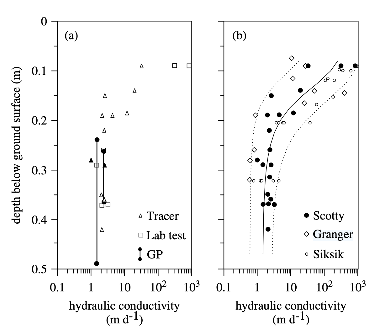
Charts of the vertical K_sat profile of peat at Scotty Creek from Quinton et al. (2008).
We're almost ready to finally see Darcy's Law written out! There is just one more piece to discuss. Darcy's Law is intended to be applied between two points in space, thus we don't strictly report on the hydraulic head at one location. Instead, we calculate a term called the hydraulic gradient. This is simply the difference in hydraulic head at two points divided by the distance between those points. Accounting for the distance between these points is critical as it indicates the steepness of the gradient. For example, a head difference of 10m is dramatic over a distance of 1m, but very subtle over 1000m. With this we can finally see Darcy's Law written out:
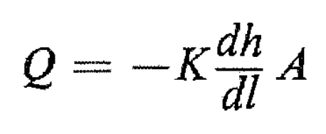
Darcy's Law per Freeze and Cherry (1979).
The resulting value, q, is known both as the Darcy flux and specific discharge, and is the volumetric flow rate of water per unit cross-sectional area of a medium. It's important to note that this is not the actual velocity of the water particles moving through a medium, but rather a "bulk" velocity representing flow through an entire cross-section of soil. The actual pore water velocity is faster than specific discharge.
One small but important nuance: because the model integrates K over the full depth of the saturated column to compute transmissivity (see below) before multiplying by the hydraulic gradient, what we're ultimately reporting is flow per unit width of the transect rather than flow per unit cross-sectional area. This gives q units of m²/d rather than m/d, so we can think of it as the total lateral discharge through a one meter wide strip of peat, summed across all depths.
I'm sure your natural next question would be: so what? Why use specific discharge instead of the actual velocity of water molecules through the soil matrix? The answer is not going to be particularly satisfying, but the truth is that it is more practical. It is much easier to measure total discharge and cross-sectional area than it is to discern pore-scale geometry. It may not reflect "true" molecular-scale velocity of water, but it is a reliable method for representing groundwater flow in mass balance calculations.
Finally, the Model
One of the challenges in modeling peatland groundwater flow is that K is not a single value, rather it varies in orders of magnitude over just a few centimetres of depth. In a uniform medium you can plug K directly into Darcy's Law and call it done. In peat, you need a way to represent the full vertical profile of conductivity and integrate it into a single flow estimate.
The model above does this using the depth-dependent K function established by Quinton et al. (2008), which describes K as a continuous curve from the ground surface down to the frost table:

The equation for K(z) provided in Quinton et al. (2008).
This equation incorporates three key points in the vertical peat profile in a single expression: very high K near the surface (approaching K_top = 360 m/day), a steep drop through the transition zone centered around z_trn = 0.15 m, and a low asymptotic value in the decomposed lower peat (K_btm = 1.4 m/day). The shape parameter n controls how abruptly that transition occurs.
Sorry to be redundant, but you can't use a single K value to apply Darcy's Law to a peat profile that is so variable. Thus, we need to rely on transmissivity (T), which is the depth-integrated hydraulic conductivity of the entire saturated column. In simple terms, it is the sum of each K layer's lateral flow contribution over the entire depth profile, and ultimately represents the total capacity of the peat column to convey water laterally.
To get a true transmissivity value I would need to integrate the equation from Quinton et al. (2008). Let's do an exercise in empathy: look at that equation, start thinking about how would integrate it, and then imagine you took calculus 6 years ago. Hopefully you can now understand why I've chosen to instead do a poor woman's transmissivity. I used Python to calculate K at the midpoint of a couple hundred thin horizontal slices of the depth profile, and then added them all together at the end. Finally, I slapped that jerry-rigged T value right into Darcy's Law and called it a day.
When you enable the ash pore-clogging toggle in the model, the K(z) parameter set shifts to reflect the findings of Ackley et al. (2021), who studied a low-severity wildfire at Scotty Creek. Despite minimal ground surface damage, Ackley measured a dramatic reduction in saturated hydraulic conductivity below roughly 10 cm depth.
The mechanism at play here is not combustion of the peat itself, but ash clogging up the peat pores. Fine ash and char particles generated at the surface are flushed downward by infiltrating water and lodge in pore spaces deeper in the profile. Ackley et al. confirmed this through pore size distribution curves, ultimately determining that effective porosity at 15 cm was 52% lower in the burned cores.
In terms of the Quinton et al. (2008) framework, this can be approximated by shifting the transition zone, or z_trn in our equation, upward from 0.15m to 0.08m. This is because the dramatic K reduction now begins closer to the surface rather than at 15–20 cm as is true in unburnt peat at Scotty Creek. I also reduced K_top in alignment with the results from Ackley et al. (2021), since the near-surface pore network is at least partially clogged. The practical consequence is a significant reduction in transmissivity, because the high-K surface layer, which would normally dominate T, is thinner. Less T means less Darcy flux for the same gradient, which is consistent with Ackley's observation that burned plateaus drained more slowly, sustained higher water tables, and showed longer pore water residence times.
The effects of pore-clogging are an optional addition, however if you click the Post-Fire option you also have the ability to specify a burn depth. Seeing as peat would burn from the top down, the model just starts the K profile at the specified depth, effectively "cutting off the top". For example, if the burnt depth is 0.2m, the K value at the ground surface will now be what was traditionally at 0.2m according to the Quinton et al., (2008) profile.
Drought scenarios in the model draw on Zhao & Jommi (2022), who subjected sphagnum peat samples to drying periods of increasing duration and tracked how it responded. Their central finding is that peat doesn't respond to drying in a simple linear way, rather there are two distinct regimes. Be warned: there is a fair bit of hand-waving in the precise selection of values ahead, but I've tried to preserve the general impacts these changes would have on the K profile established in Quinton et al. (2008).
In the first moderate drought regime, drying compresses the large pores. Counterintuitively, K was barely affected, or can even increase slightly, because as the peat matrix consolidates, new cracks form and macropores enlarge. The fibrous network remains largely intact. In the model, this impact is incorporated by expanding the upper, highly conductive layer of peat. K_top stays at its baseline value, but the transition zone shifts slightly deeper.
In the second, more rigorous drought regime, the plant fibers themselves begin to desaturate. This is an almost irreversible process in which organic components become progressively hydrophobic, the cellular structure within the peat fibers collapses, and they break into shorter fragments. The result is a dramatic, permanent loss of the large connected pores that drive high K. Zhao & Jommi found K dropped by orders of magnitude once this drying threshold was crossed. The model's severe drought scenario tries to emulate this collapse. To start, K_top drops from 360 to 30 m/day. This is because in Quinton et al. (2008), 30 m/day is the lowest K_top observed through their field data collection. Therefore, this value seems plausible and would be reflective of a collapsing upper peat pore network. I additionally reduced K_btm by about half, bringing it down from 1.4 to 0.7 m/day, again to reflect the collapsing peat structure. Additionally, I "smoothed" out the transition curve (n parameter) from 4.3 to 3.0 to reflect the loss of that stark highly conductive layer that creates the more dramatic shape of the original Quinton et al. (2008) curve.
Post-drought recovery is represented by a partial restoration of all parameters (for example, K_top goes recovers to 100 from 30 m/day). The cumulative drought condition represents a multi-year gradual fibre degradation without a single catastrophic threshold crossing. This is applied here via a modest (and theoretically progressive, although this model is just a single snapshot in time) decay from 360 to 300 m/day. All other parameters are left the same with the idea in mind that in continuous, mild drought conditions the bottom layers of peat would likely stay more saturated than the near-surface layers.
Here's how each of the scenarios modifies the original K_sat profile from Quinton et al. (2008):
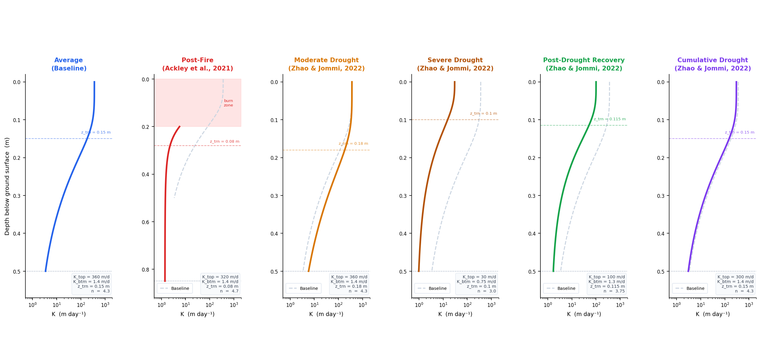
The modified K_sat profiles for each of the disturbance scenarios.
For each scenario, the simulator selects the appropriate K_top, K_btm, z_trn, and n, then:
- Evaluates K(z) at each depth increment across the active layer using Quinton's equation
- Numerically integrates K(z) over the saturated column to compute T
- Computes the hydraulic gradient i from the water table depths at each end of the transect divided by the horizontal distance L
- Multiplies T × i to produce the depth-integrated Darcy flux q, displayed at the top of the cross-section
The color shading in the diagram reflects K(z) at each depth, and is anchored to the full Quinton baseline range so you can see directly how each scenario reshapes the vertical conductivity structure. The flow arrows scale with local q at each depth layer, illustrating how the shallow, high-K peat dominates lateral flow under baseline conditions, and how that flow profile erodes under fire or drought disturbance. Scroll to the bottom for citations.
Phew, that was a doozy! My morale is saved by a new Olivia Rogrido drop on this day in history. For your viewing pleasure:
References
Ackley, C., Tank, S. E., Haynes, K. M., Rezanezhad, F., McCarter, C., & Quinton, W. L. (2021). Coupled hydrological and geochemical impacts of wildfire in peatland-dominated regions of discontinuous permafrost. Science of The Total Environment, 782, 146841. https://doi.org/10.1016/j.scitotenv.2021.146841
Freeze, R. A., & Cherry, J. A. (1979). Groundwater. Prentice-Hall.
Quinton, W. L., Hayashi, M., & Carey, S. K. (2008). Peat hydraulic conductivity in cold regions and its relation to pore size and geometry. Hydrological Processes, 22(15), 2829–2837. https://doi.org/10.1002/hyp.7027
Zhao, H. F., & Jommi, C. (2022). Consequences of drying on the hydro-mechanical response of fibrous peats upon compression. Canadian Geotechnical Journal, 59(10), 1712–1727. https://doi.org/10.1139/cgj-2020-0086